Simulating the Microlife Macrolife and the Galaxy
[Fall 2022] Our project is a particle simulation controller that uses a graphical interface and a joystick to interact with a user-defined set of particle interactions.
- Suitable forB.Tech/B.E Embedded Systems students
- Build time4-6 weeks
- LevelBeginner
- Available atAjvika Labs, Kakinada
About this project
Clusters
Simulating the Microlife, Macrolife, and the Galaxy
Made by
Introduction
Our project is a particle simulation controller that uses a graphical interface and a joystick to interact with a user-defined set of particle interactions.
For the final project, our goal was to simulate unique particle interactions using a clustering algorithm that operates at a speed of at least 20 FPS. There are user-defined sets of particles (groups) that all share the same properties.
The user has two ways to interact with the particles: they can use the interface to influence the particle interactions between each of the particle groups and they can use an interactive joystick to directly modify the positioning and behavior of the particles. The joystick controller is not meant for precise particle interactions, but to simulate a sudden disruptive external force entering the system.
The result of these simple interactions ranged from a potentially distinctive clustering behavior to a chaotic, forever-moving behavior with no steady state.
This project is intended to be an interactive plaything, but during testing we found several applications that it could be used for. While it could be used as a fun game for many people, it could also be used as an educational tool simulation. Although real life particles operate under more complicated equations, this simulation could still be used to demonstrate how atomic particles, and even how organic bodies, interact.
High Level Design
The motivations behind this final project were derived from Lab 2's particle lab that simulated the movement of animal groups. We were inspired by the surprisingly unique results that could arise from a set of relatively simple equations. As a result, we decided to create
Clusters
, which builds on the same idea of particle interactions, but generalizes the equations to display a much wider range of particle behaviors. We decided to use the interactive principles of gravity to achieve this goal. To have a set standard of correctness, we also used the following website online, which relies on similar principles:
Particle Life
. Having a standard is important for a project like this because it is not entirely clear what the expected behavior should be at all times, even for the designers. By modifying our values to be the
theoretical
equivalent of
Particle Life's
, we could discern where potential errors might have been made.
Background Physics and Math
In order to create our particle system, we needed an acute understanding of how forces are created between two masses and how those forces influence the moving behaviors of those bodies. The forces that we are considering in this closed environment are the forces of gravity and drag force. Both have nontrivial involvement towards the velocities and the positions of particles in the real world, as such, a physics and math background greatly expedited our implementation.
Gravitational Force
It is said that 2 bodies of any mass exert the same gravitational force on one another. For example, as the Earth pulls down on us with gravity, we exert our own "gravity" on the Earth that pulls it up towards us. The force from us and the force from the Earth are exactly the same. The only significant difference is the change in speed (
acceleration
) that this same force causes on 1 body vs the other. We take advantage of this property to greatly simplify our calculations.
Original gravitational force equation (above) and its reworked counterpart (below)
If we take every particle's mass to be the same (1 for simplicity), we only need to modify the G constant so it accounts for that interaction between two masses. However, if the masses are the same
and
the forces are the same, then, the acceleration would be the same for two particles, no matter their true respective masses. To solve this, we simply allocate two G constants for the same interactions between 2 particles. As such, the gravitational constant of particle A on B will not be the same as B on A! By removing the bidirectional nature of force, we can combine the mass ratios of particle A, particle B, and the gravitational constant all into a single constant!
To take it a step further, we consider a force with linear decay with respect to distance as opposed to exponential decay. We could still portray similar behaviors even without an accurate decay rate, so we opted for this path for optimization.
Drag Force
Drag force is the force that acts on bodies that do not travel in the same velocity as the environment. For example, if the velocity in an environment is 0, it will simply act against any type of motion. This can be seen with skydivers, whose bodies will eventually stop accelerating because the drag force acts against the force of gravity. This force depends on the drag coefficient, C, the density of the "fluid", p (air, water, a vacuum, etc), and the cross-sectional area, A, in the direction of the mass velocity, v.
Original drag force equation (above) and its reworked counterpart (below)
As before, we can combine many of the constants into a single constant variable that represents the behavior of the entire environment. This suggests making the assumption that the particles all have the same area, but not much is lost in this assumption. Since we are displaying each particle with the same amount of pixels, this is much easier to visually accept. Furthermore, having the same area does not imply different masses, so it does not conceptually contradict the gravitational force manipulations.
We also removed the exponential factor from the velocity and made it linear instead. As before, this was done for optimization purposes and does not have huge ramifications on the visual behavior of the particles since this is a more secondary, reactive force.
Logical Structure
The modifications to the fundamental physics equations above guided our program's control flow and our logical structure as seen below.
A diagram of particle-to-particle interactions. The grayed out boxes are ignored interactions.
Our program uses each of the constants previously defined to change the state (position and velocity) of each particle. It does this by iterating through each particle in a twice-nested loop. First, each particle must check the distance between itself and the corresponding particle. If this distance is greater than a set visual range, then the interaction fails and the particle is unaffected by it. If it is within the acceptable range, then interaction calculations can proceed. Each particle is able to then "collect" the gravitational influence that the other particles impose on it and move to the correct x and y position accordingly.
As stated before, the interactions work in such a way such that the A->B interaction will look completely different from the B->A interaction. Particle A and particle B will each belong to a subclass of groups with their specified interactions with other groups. A and B could belong to different groups or potentially the same group with the same interaction! Furthermore, it is undefined behavior for a particle to interact with itself, so that situation is always ignored as well.
Like each particle, the joystick also has a "visual range". Whenever it is pressed, the particles inside this visual range will be immediately pushed outside its radius, ignoring any previously accumulated forces. We designed the joystick in this manner so the user could directly enter the
closed system
and add their own external forces. Furthermore, it was to have a way to precisely interrupt steady state behaviors to observe how the system recovers from external stimuli.
Software Tradeoffs
While implementing our optimizations to spawn more particles, we discovered that there was a very apparent tradeoff between accuracy and performance. For example, we eased the calculation rate of the particles such that for each iteration, a fraction of the particles would be ignored for calculations. This allows us to significantly improve our framerate, but as a result, the interactions between particles are loose and chaotic, at best.
The more calculations we forgo, the more loose the interactions are, until the particles appear to act independently of one another. Unlike previously observed, this situation prevents any type of steady state behavior such as clustering or equilibrium. We settled for a ratio of about one third. That is, 1 out of every 3 particles will not be considered for every iteration. This was the golden ratio that we acquired through trial and error. With one third ignored, we still saw the expected steady state patterns, but with the added benefit of being able to spawn
more
particles.
UI Display
Our finalized UI design, created in python. Each of the colors represents a valid group of particles. Changing the G slider on the bottom alters the group-to-group interactions of the particles. The values on the left changes the environmental variables as well as some environmental constants.
Program and Hardware Design
We are running two programs for this project. One of these programs is a C program running on the Raspberry Pi Pico, and the other is a Python program running on a computer. The C program is responsible for doing all of the particle calculations, displaying the particles on the VGA screen, reading and incorporating the joystick values, and reading and incorporating values from the serial terminal. The Python program is responsible for running the GUI and sending any changes that the user makes to the C program through the serial terminal.
The C program uses two threads. The first thread draws the particles and the text on the VGA screen. It also reads and processes data from the serial port. The second thread performs all calculations for updating the positions and velocities of the particles. Since the two threads are doing very different things, we did not need to worry
Technologies used
Hardware components
- Raspberry Pi Pico
- IMU
Software & tools
- Python
Project demo video
What you get
- Working project / hardware kit, tested before delivery
- Complete source code with explanation
- Project demo and guidance for your viva
- Project report, PPT and IEEE paper support (on request)
Delivery & Payment
Delivery takes a minimum of two weeks from the date your inquiry is confirmed.
Payment is in two parts:
• 50% advance to start the project
• Remaining 50% before delivery
Note:
• Documentation and PPT are not included by default
• If you need documentation/PPT, it can be arranged for extra time and cost
We'll confirm the exact timeline and cost with you after reviewing your requirements.
Related Embedded Systems projects
Embedded Systems
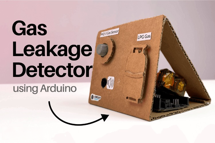
Gas Leakage Detector Using Arduino
A budget-friendly LPG gas leak detector built with an Arduino and MQ-5 gas sensor, triggering a buzzer and LED when unsafe gas levels are de...
View project
Embedded Systems
Simple Alarm System
A beginner-friendly home alarm with PIR motion sensing, keypad PIN entry, and separate entry/exit timing delays, built to be easy to expand.
View project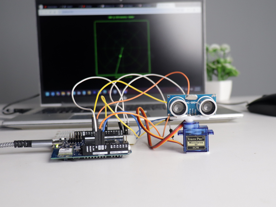
Embedded Systems
Ultrasonic Sensor Project with Arduino UNO Q
A beginner-friendly first Arduino UNO Q project: a servo-swept ultrasonic sensor that renders a live sweeping radar display in a web browser...
View project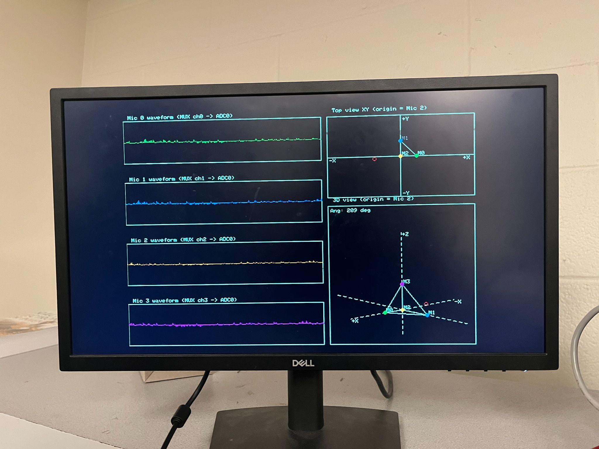
Embedded Systems
3D Audio Localization
[Fall 2025] We designed a real-time embedded system that localizes sound sources in three dimensions and visualizes them live using a four-m...
View project