3D Audio Localization

ECE 5730 - Final Project Report
Demonstration Video on YouTube
1. Project Introduction
We designed a real-time embedded system that localizes sound sources
in three dimensions and visualizes them live using a four-microphone
array and a VGA display. The system uses time-difference-of-arrival
(TDOA) estimation, cross-correlation, and a grid-search-based solver
on a Raspberry Pi Pico to compute sound source positions in real time,
with the goal of making sound localization more interpretable by
directly mapping acoustic timing differences to intuitive 2D and 3D
visual feedback.
2. High Level Design
2.1 Rationale and Motivation
Sound source localization is a fundamental problem in signal
processing and embedded systems, with applications in robotics,
human–computer interaction, and spatial sensing. In many
implementations, however, localization results are presented only as
numerical estimates or offline plots, which makes the behavior of the
system difficult to interpret. The primary motivation of this project
was to design a real-time embedded sound localization system that
provides intuitive visual feedback, allowing users to directly observe
how acoustic signals map to spatial position estimates. By combining a
four-microphone array with time-difference-of-arrival (TDOA)
estimation and live VGA visualization, this project turns sound
localization into an interactive and observable process.
The system was designed to align closely with the core themes of the
course, including real-time embedded computation, multi-core
concurrency, signal processing, and graphical visualization. Four
microphone channels are sampled at 10 kHz, and acoustic events are
detected and processed to compute six pairwise TDOA measurements.
These measurements are used to estimate a three-dimensional sound
source position, which is then displayed in real time as both a 2D
top-down view and a rotating 3D visualization. At the same time, raw
microphone waveforms are shown on the display, enabling direct
correlation between the input signals and the resulting localization
output.
This project was conceptually inspired by prior course projects that
explored microphone-array-based sound localization and real-time
visualization on embedded platforms, particularly the Spring 2025 ECE
4760/5730 project "
Audio Localization with Raspberry Pi Pico
" developed by Sam Belliveau et al. That project demonstrated
event-based audio detection and spatial estimation using multiple
microphones. Building on these ideas, our work extends the approach
toward full three-dimensional localization and improved spatial
interpretability. Specifically, we employ a four-microphone array to
estimate six pairwise time-differences-of-arrival (TDOAs) and recover
a 3D sound source position using a grid-search-based formulation. In
addition, the system provides continuously updated VGA visualization
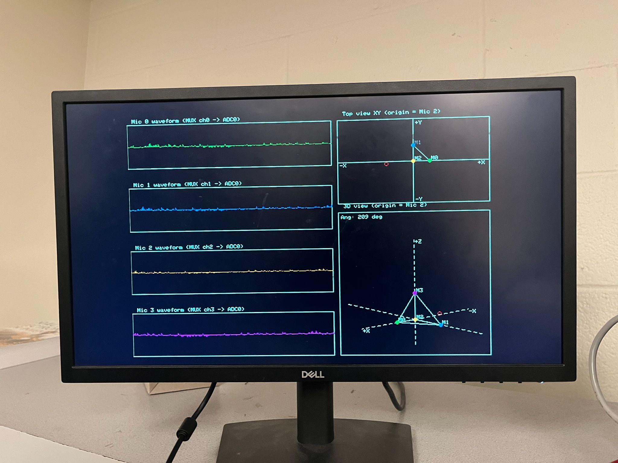
that integrates raw microphone waveforms with both 2D and rotatable 3D
spatial views, allowing users to directly observe how acoustic timing
differences map to estimated source locations.
Building on these ideas, our work extends the approach toward full
three-dimensional localization and improved spatial interpretability.
Specifically, we employ a four-microphone array to estimate six
pairwise time-differences-of-arrival (TDOAs) and recover a 3D sound
source position using a grid-search-based formulation. In addition,
the system provides continuously updated VGA visualization that
integrates raw microphone waveforms with both 2D and rotatable 3D
spatial views, allowing users to directly observe how acoustic timing
differences map to estimated source locations.
Figure 1: VGA Visualization of Microphone Position and Input
2.2 Background Math
Sound source localization using a microphone array exploits the fact
that an acoustic wave reaches spatially separated microphones at
different times. These time differences depend on the microphone
geometry and the three-dimensional position of the sound source, which
is modeled as an unknown point $\mathbf{s} \in \mathbb{R}^3$. The
microphone positions $\mathbf{m}_i$ are assumed to be known and fixed.
Under free-field propagation and assuming a constant speed of sound
$c$, the signal arrival time at microphone $i$ is modeled as:
$$t_i = t_0 + \frac{\|\mathbf{s} - \mathbf{m}_i\|}{c}$$
Here, $t_0$ is the unknown emission time of the sound event. Because
this emission time is not observable, absolute arrival times cannot be
directly used for localization.
To eliminate the unknown emission time, time-difference-of-arrival
(TDOA) measurements are computed between microphone pairs. For
microphones $i$ and $j$, the TDOA is defined as:
$$\Delta t_{ij} = t_i - t_j$$
Substituting the propagation model into the TDOA definition yields:
$$\Delta t_{ij} = \frac{\|\mathbf{s} - \mathbf{m}_i\| - \|\mathbf{s} -
\mathbf{m}_j\|}{c}$$
This expression directly relates the unknown source position to
measurable time delays. With four microphones, six independent
microphone pairs provide sufficient constraints for three-dimensional
localization.
In a sampled system, TDOAs are estimated from discrete-time microphone
signals using cross-correlation. For signals $x_i[n]$ and $x_j[n]$,
the cross-correlation function is defined as:
$$R_{ij}[k] = \sum_n x_i[n] \, x_j[n + k]$$
The estimated delay corresponds to the lag that maximizes the
magnitude of the cross-correlation:
$$\hat{k}_{ij} = \arg\max_k |R_{ij}[k]|$$
The corresponding TDOA estimate is obtained by converting the lag to
time using the sampling frequency $f_s$:
$$\hat{\Delta t}_{ij} = \frac{\hat{k}_{ij}}{f_s}$$
To estimate the source position, a least-squares grid search is
performed over a discrete set of candidate locations $\mathbf{s}_g$.
For each candidate, the predicted TDOAs are computed as:
$$\Delta t_{ij}^{(g)} = \frac{\|\mathbf{s}_g - \mathbf{m}_i\| -
\|\mathbf{s}_g - \mathbf{m}_j\|}{c}$$
An error function is constructed by summing the squared differences
between measured and predicted TDOAs:
$$E(\mathbf{s}_g) = \sum_{i \lt j} \left( \hat{\Delta t}_{ij} - \Delta
t_{ij}^{(g)} \right)^2$$
The estimated sound source position is selected as the grid point that
minimizes this error function:
$$\hat{\mathbf{s}} = \arg\min_{\mathbf{s}_g} E(\mathbf{s}_g)$$
2.3 Logical Structure
Figure 2: An Overview of the Software Design
The software is divided into three main subsystems that run across the
RP2040’s interrupt handler, two protothreads, and a VGA rendering
core.
The timer-based ISR samples four microphones through a CD4051B
multiplexer at 10kHz. In each sampling, ISD stores the data in ring
buffers, tracks signal energy, and triggers a TDOA event when all
microphones detect a sound at nearly the same time. The
protothread_tdoa task then copies the buffered samples, removes DC,
normalizes the signals, computes cross-correlations, and performs a 3D
grid search to estimate the sound source position. The
protothread_angle task reads a potentiometer and applies low-pass
filtering to determine the viewing angle for visualization. Core 1
handles all VGA drawing, including microphone waveforms, a 2D XY map,
and a rotatable 3D view that uses shared state from the main core.
2.4 Hardware / Software Tradeoffs
A key design tradeoff in this project involves the choice of audio
sampling rate versus computational load. A sampling rate of 10 kHz was
selected as it provides sufficient temporal resolution to resolve
inter-microphone delays on the order of a few milliseconds, which is
appropriate for the physical spacing of the microphone array. With a
maximum correlation lag of ±30 samples, the system can capture up to
±3 ms of arrival-time difference while keeping the interrupt service
routine and downstream processing manageable. Higher sampling rates
would increase timing precision but would significantly raise
interrupt frequency and processing overhead, making real-time
operation more difficult on the RP2040.
Another important tradeoff is between continuous localization and
event-triggered computation. Rather than performing cross-correlation
and localization continuously, the system uses energy-based detection
to identify salient acoustic events and only performs TDOA estimation
when all four microphones detect an event within a short time window.
In addition, a minimum interval of 0.1 seconds is enforced between
successive localization events. This strategy greatly reduces
unnecessary computation, prevents repeated triggering from echoes or
sustained noise, and ensures that expensive operations such as
cross-correlation and grid search do not overwhelm the processor.
The choice of a grid-search-based localization algorithm represents a
tradeoff between computational efficiency and robustness. Closed-form
geometric solutions or lookup-table-based approaches can be efficient
under ideal conditions but tend to be highly sensitive to measurement
noise, synchronization errors, and modeling inaccuracies. In contrast,
a grid search evaluates a physically meaningful error function over a
finite spatial region and selects the position that best matches the
observed TDOA measurements. Although this approach is computationally
more intensive, it is simple to implement, tolerant of noise, and
well-suited to an event-driven execution model on an embedded system.
We adopt a dual-core architecture to keep visualiza