ScopeBoy Handheld Mixed-Domain Oscilloscope

ScopeBoy
v1.0
Final Report
Project Introduction
One-sentence sound bite
Summary (what you did and why)
High Level Design
Rationale & sources of idea
Background math
Logical structure
Hardware/software tradeoffs
Relevant patents/copyrights/trademarks
Program / Hardware Design
Program details
Hardware details
Reused code/design
Things that did not work
Thorough discussion of AI use
Results of the Design
Test data / traces / waveforms
Speed of execution
Accuracy
Safety enforcement
Usability
Conclusions
Expectation vs results / next time
Applicable standards
Intellectual property considerations
Appendices
Appendix A: Permissions
Appendix B: Program listings
Appendix C: Schematics
Appendix D: Team member tasks
References
ScopeBoy: Handheld Mixed-Domain Oscilloscope (MDO)
Project:
ScopeBoy: Portable Oscilloscope
Team:
Robbie Leslie, Immanual Koshy
Course:
ECE 5730
Date:
December, 2025
Project Introduction
This project builds ScopeBoy, a handheld, dual-core mixed-domain oscilloscope (MDO) on the Raspberry Pi Pico RP2040,
featuring real-time spectral analysis and gain control.
Using the RP2040 microcontroller, we created a device that samples signals at 500 kSps. It leverages the dual-core
architecture to separate signal processing (FFT math) from the user interface (drawing waveforms), ensuring a lag-free 60 FPS
experience.
Key Features
Oscilloscope Mode:
Adjustable timebase (10ms-1s), voltage scale, and live cursors.
Spectrum Analyzer Mode:
64-bin real-time FFT with Hanning windowing and peak frequency detection.
Easter Egg:
A fully playable "Snake" game triggered by a hidden button combo.
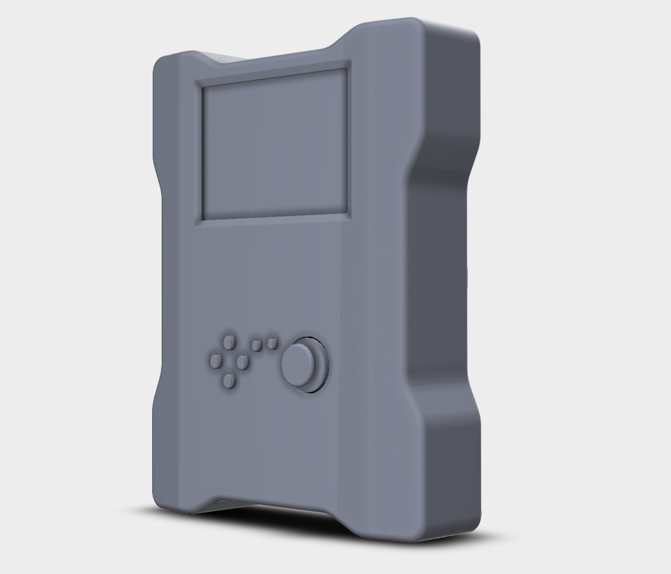
ScopeBoy 3D Render - Assembled Device Concept
Project Demo Video
High Level Design
Rationale and sources of your project idea
We wanted a portable, battery-friendly instrument for quickly debugging real-world signals (especially PWM control signals and
small audio circuits) without needing a bench scope.
Motivation / constraints:
A handheld tool that is fast to deploy for labs, demos, and quick iteration,
while still providing both time-domain and frequency-domain visibility.
Inspiration:
The Cornell ECE4760/ECE5730 course structure and prior RP2040 oscilloscope projects motivated a
dual-core approach that keeps the UI responsive while running DSP in parallel.
Background math
Nyquist-Shannon Sampling Theorem:
With a sampling rate of 500 kSps, the highest measurable frequency
without aliasing is 250 kHz (the Nyquist frequency).
Discrete Fourier Transform (DFT):
Our
computeDFT()
converts a block of \(N\) time samples
into frequency bins:
X_k = Σ_{n=0}^{N-1} x_n · e^{-j2πkn/N}
Where:
x_n
is the input voltage sample at index
n
X_k
is the output spectral component (magnitude and phase) at frequency bin
k
We compute real/imaginary components and then convert to magnitude, \( |X_k| = \sqrt{Re^2 + Im^2} \), to find peaks.
Windowing (Hanning Window):
Because we capture a finite “slice” of a continuous signal, the start and end
of the sample buffer rarely align perfectly. This discontinuity causes
spectral leakage
, where energy from one
frequency bleeds into neighboring bins. We apply a Hanning window before running the FFT/DFT to taper the edges:
w(n) = 0.5(1 − cos(2πn/(N−1)))
Logical structure
The system uses an Asymmetric Multiprocessing (AMP) model to ensure the User Interface (UI) never stutters, even when
performing heavy calculations.
Create a block diagram showing:
Core 0 (The Application Processor):
Responsibilities:
Handles all User Input (Joystick, Buttons, Rotary Encoder), manages the Trigger Logic
(detecting rising/falling edges), and drives the SPI TFT Display.
Architecture:
Runs a cooperative scheduler (
protothreads
) to toggle between input polling
and screen rendering at 60Hz.
Core 1 (The DSP Coprocessor):
Responsibilities:
Dedicated entirely to number crunching. It runs an infinite loop that waits for fresh
data, applies the Hanning Window, computes the DFT, and updates the FFT output array.
Benefit:
Because this math happens on a separate core, the oscilloscope trace on screen never “freezes”
or lags, even if the math takes milliseconds to complete.
Shared Memory & Synchronization:
The
frame_buf
(ADC samples) and
fft_output
arrays reside in shared RAM.
Access is managed via flags and semaphores to ensure Core 1 doesn't try to calculate the FFT while Core 0 is
simultaneously writing new data from the ADC.
Hardware/software tradeoffs
1. Signal Processing (FFT): Software (Core 1) vs. Dedicated DSP Hardware
Decision:
Implemented
Software FFT
on the secondary Cortex-M0+ core.
Performance:
While a dedicated DSP chip or FPGA would calculate DFTs microseconds faster, the RP2040's dual-core
architecture allowed us to offload the math to Core 1. This prevents the UI (Core 0) from freezing, achieving a "good enough"
real-time update rate (approx. 15-30 Hz for FFT) without additional hardware.
Cost & Complexity:
Using the existing microcontroller reduced the Bill of Materials (BOM) cost by ~$5-10 and
significantly reduced PCB complexity.
Maintainability:
Doing the math in C allows for easy adjustments to windowing functions (e.g., swapping Hanning
for Blackman) without rewiring hardware.
2. Analog Front End: Digital Zoom vs. Analog Gain
Decision:
A
Hybrid approach
. We use hardware switches (Gain Modes) for coarse range adjustment, refined by software scaling.
Performance:
Purely software "zoom" (multiplying the ADC value) destroys signal resolution; zooming 10x on a 10mV
signal amplifies the quantization noise. Hardware gain (using Op-Amps/Relays) preserves the Signal-to-Noise Ratio (SNR) before it
hits the ADC.
Complexity:
Adding hardware gain stages increases circuit complexity and power consumption compared to a simple
voltage divider, but it was strictly necessary to measure small signals accurately.
3. Display Driving: Hardware SPI vs. Bit-Banging
Decision:
Hardware SPI Peripheral
Performance:
Driving a 320x240 display requires pushing ~153,000 bytes per frame. "Bit-banging" (toggling pins in
software) would cap the frame rate at ~5 FPS. Using the RP2040's hardware SPI block allows us to reach 60 FPS with minimal CPU
overhead.
Power:
Hardware peripherals are more power-efficient as they allow the CPU to sleep or perform other tasks (like
polling inputs) during data transmission.
Program / Hardware Design
Program details
This project required solving several complex graphics and concurrency problems to achieve a stable 60 FPS update rate on the
RP2040.
Program Details: Technical Challenges & Solutions
1. The "No-Fly Zone" Rendering Algorithm
One of the most persistent issues in digital oscilloscope displays is text flickering or overwriting. If the waveform is drawn
across the entire screen width, it inevitably scribbles over the voltage axis labels (e.g., "3.3V", "1.65V") on the left
side. Redrawing these labels every frame is computationally expensive and causes flashing.
The Solution:
We implemented a viewport clipping algorithm in the
drawWaveformFromBuffer
function. By defining specific
WAVE_MARGIN
constants (Left: 35px, Top: 25px, Bottom: 20px), the renderer
creates a "protected" area for the UI.
How it works:
The drawing loop starts at
x = MARGIN_LEFT
rather than

. Any
signal sample that exceeds the vertical bounds (
MARGIN_TOP
or
MARGIN_BOTTOM
) is mathematically
clamped before drawing. This ensures the waveform "emerges" cleanly from behind the axis labels without ever corrupting the
text pixels.
2. Flicker-Free Graphics (Smart Erase)
Standard graphics libraries often rely on
tft_fillScreen(BLACK)
to clear the frame before redrawing. On SPI
displays, this bulk pixel transfer is too slow and results in a visible "scanline" flicker.
Snake Mode Implementation:
Instead of clearing the screen, we used a
differential rendering
strategy. The game logic tracks the exact position of the snake's tail before it moves. We draw a single black block over the
old
tail position and a colored block at the
new
head position. This reduces the SPI bus load from
~76,000 pixels per frame (full screen) to just ~200 pixels per frame.
Oscilloscope Grid:
Similarly, when the waveform erases its old trace (drawing black lines), it often
accidentally deletes the grid lines. We added a "Repair Bot" logic inside the draw loop: if the eraser crosses a known grid
coordinate (e.g.,
x=160
or
y=120
), the function immediately repaints that specific grid pixel,
maintaining a solid, unbroken reticle.
3. Dual-Core Concurrency
The RP2040 features two ARM Cortex-M0+ cores, which we leveraged to separate the real-time blocking tasks from the math-heavy
processing.
Core 0 (The Interface):
Runs the
protothreads
scheduler to handle high-speed SPI display
rendering and user input (Joystick/Buttons). This ensures the UI remains responsive (60 FPS) at all times.
Core 1 (The Math Coprocessor):
Dedicated solely to the FFT calculations. Using
multicore_launch_core1
, this core continuously processes the ADC buffer, applying the Hanning window and
computing the Discrete Fourier Transform (DFT).
Synchronization:
Shared memory access to the
frame_buf
array is protected using semaphores to
prevent race conditions (read-while-write errors).
4. Rotary Encoder
The rotary encoder generates pulses on its CLK and DT pins when rotated. The direction is determined by looking at if the pulse on CLK or DT was first. Professor Bruce had previously worked w