Pandoras Box Epidemic Simulator

Pandora’s Box
Project Introduction
Our final project is a stochastic, agent-based epidemic simulator with adjustable parameters through physical sliders and displayed via VGA on a 640 x 480 screen alongside statistical graphs demonstrating the spread of the disease.
Project Summary
Epidemic simulations can be divided into two broad philosophies: deterministic SIR (Susceptible-Infected-Recovered) models and stochastic agent-based models. In SIR models, differential equations are matched to the desired modeled scenario, which are then solved to show the result of the epidemic. It is deterministic because the result does not change per run. An agent-based simulation prescribes behavior parameters to each agent (in our case, balls representing people), which then are simulated to interact. Some randomness is then incorporated to make each run unique, determined by each step of the simulation, thus stochastic. However, in the long run, total runs will converge to the average expected behavior.
We chose to tackle simulating an agent-based model on the RP2040’s limited hardware. We chose this over the SIR based model because we wanted to create a simulation that is both interactive and educational, allowing the user to play with the relevant parameters and observe how their combined effects can affect how an epidemic spreads, and its results. We also implement spatial (tree) and temporal (auto-scaling population distribution graph) data displays in order to better represent the larger changes in the system.
High-level Design
Rationale
We were primarily inspired by the UI/UX experience in the Youtuber 3Blue1Brown’s video on epidemic simulation, as well as our own lived experiences of the Covid-19 pandemic. We did not examine his software design so as to not plagiarize, and only aimed to create a similar UI/UX experience at the surface level.
We separate the balls into 12 color-coded, separate grids in order to simulate real-life neighborhoods/cities/countries (places of congregation). Two graphs then demonstrate the temporal and spatial changes of the simulation. The top graph is a tree graph showing how the disease spreads from person to person by generation, as well as which grid each ball is currently in. The bottom graph is a time versus population distribution graph that shows the change in percent of people who are susceptible (green), infected (red), recovered (blue) and dead (dark blue). It automatically rescales as time goes on, enabling an overall view of the simulation’s entire timeline. It can capture roughly two minutes of data.
Where we took design liberty is in the implementation, as 3Blue1Brown’s implementation was done in Python, an entirely different resource environment compared to C on the RP2040. Programs in Python run on a modern computer have access to infinite CPU resources, RAM, and program memory relative to the RP2040. Our program must be efficiently designed, conservative in memory usage, and concisely coded. This was a key focus from the start, as we did not know to what degree the RP2040 could actually simulate something similar to the video’s model. For a project of this scope, essentially no hardware/software tradeoffs have to be considered in Python (within reasonable limits), so it was not designed at all with the RP2040 in mind.
Background Math
There are a diverse number of individual methodologies as to designing agent-based epidemic models. We chose to employ a combination of simple probability measurements, as well as collision physics simulations to model our parameters. The choice of using balls moving around in grids is, as mentioned prior, sourced from 3Blue1Brown’s design in his video. We then model human movement within a community as ball interactions, allowing us to use modified collision physics simulation code to model our various parameters.
Collision physics simulation can easily be modified to simulate a variety of other effects when its structure is examined. Fundamentally, it is an event that triggers when a ball is within a certain distance of another ball. By altering the event, involving probability as to if the event can occur, and assigning unique distances for each event, we can simulate all our desired parameters. We employ this setup for calculating infections, social distancing, and ball-wall collisions.
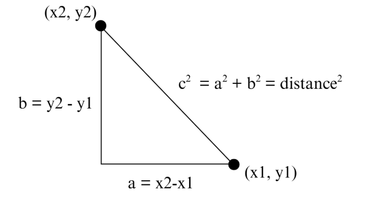
The traditional approach to calculating distance is using the Pythagorean Theorem.
By keeping track of each ball’s \( x \) and \( y \) coordinates in terms of which pixels their centers are occupying, we can calculate the distance between balls as prescribed in the above diagram. However, because we expected efficiency and memory to be our #1 issue, we decided to instead use the alpha beta approximation in order to avoid multiplication of large numbers.
The alpha beta approximation states that the sum of two squared values, and therefore distance squared
\[
= a^2 + b^2 \approx \alpha \cdot \mathrm{Max} + \beta \cdot \mathrm{Min}
\]
, in which \( \alpha \) and \( \beta \) are set constants, Max is the larger absolute value between \( a \) and \( b \), while Min is smaller. We then only need to compare this to the relevant radius (infection, social distancing, etc.) squared to determine if two balls (or a ball and a wall) are within distance.
All probability parameters are done using simple division. We randomly generate a number between a chosen range (which is different for each parameter to create a realistic model) and if it is below the parameter probability, then the event occurs (say, death). The exact determination of what constitutes an “accurate” range was not calculated, but intuited based on our observations.
The reasoning for this choice is, for one, because it is relatively difficult to precisely model the actual probability of any given event. In our design, we are checking for infections/death etc. at \( 3\,\text{Hz} \). We picked \( 3\,\text{Hz} \) after trial and error, finding it to limit the epidemic to a desirable time frame (within a few minutes), and effectively demonstrate each parameter’s effects without things changing too fast/slow to be observed. The actual probability of an infection per ball-ball encounter is
\[
P(\text{at least 1 success in } n \text{ rolls})
= 1 - P(\text{no success in } n \text{ rolls})
\]
, in which
\[
P(\text{no success in } n \text{ rolls}) = (1 - P(\text{infection}))^n
\]
and \( n = \text{num} \). We can thus see that since \( 1 - P(\text{infection}) \) is always \( < 1 \) (as all probabilities are), then as the number of rolls increase, it is far more likely for a success to occur.
We could, of course, choose to ascribe the probability to only when a ball enters another ball’s radius. However, that would also be an inaccurate model, as in real life, longer exposure time, more close contact is more likely to cause disease spread compared to a brief, distant one. Furthermore, our project goal is not to create an accurate model that can precisely predict exactly how an actual epidemic would spread. Instead, it is meant to simulate the relative relationships between each parameter in an epidemic. Thus, though we picked 3Hz subjectively, it creates a constant error across all parameter’s effects. The relative relationship between parameters, however, remains the same.
Our chosen, changeable parameters are described below. Each specific implementation will be discussed further in the program design section.
Infection Radius: How close balls must be for infection to potentially occur
Social Distancing Radius: How close balls can be before they are “repelled” (modeled as collision)
Change Grid Probability: The probability for a random ball to be moved to a new grid
Infection Probability: The probability an infection successfully passes from one ball to another
Death Probability: The chance an infected ball will “die” (no longer transmitting and becomes stationery)
Some parameters that users cannot interface with currently, but are implemented in a similar fashion and could have been wired to a switch are: Vaccination Percentage, Infection Delay, Vaccination Infection Probability, and Infection Duration.
Block Diagram
Hardware-Software Design Tradeoffs
One key software trade off is whether to employ 2, 3 or 4-bit color with the VGA. Experience has shown that after sufficient optimization, the key limitation to the scale of the simulation both temporally (in terms of the graphs) and spatially (the number of balls) is a lack of memory space on the Raspberry Pi Pico board. By increasing the bits used for color, we effectively increase the space each pixel takes up in memory for ALL pixels. The easiest solution is to reduce our palette for optimization. However, we ultimately decided not to reduce our palette, and maintain 4-bit color, giving us a choice of 16 colors for animation. While optimization was important, we recognized that our goal was to provide a visualization of disease spread. The less colors we had, the harder it is to distinguish different colored traits from each other. (e.g. infected from susceptible, or which grid a ball belonged to on the tree graph) In the end, we ended up utilizing every color available, demonstrating that this was a necessary sacrifice of optimization.
Another tradeoff we decided on was which parameters are user-changeable, and which are not. The RP2040 only has 4 ADC (analog-to-digital) channels, which are required if we want to read voltage readings from slider switches to change parameters. While theoretically we could hook up a mux to each of the 4 ADC channels on the RP2040, and thus ascribe a value to each, this was not realistic for us to build within the project time frame. Due to further limitations of our enclosure, we ended up only having 5 slider switches hooked up to a single 8-to-1 multiplexor. The RP2040 then sweeps through the inputs of the external multiplexor to read 5 switches in a single ADC channel. We ultimately decided on the five we chose as the most n