License plate recognition system

Final Project Report

Introduction
We designed a proof of concept plate recognition system that automatically recognizes and release cars from the parking lot.
Machine learning algorithms are becoming more prevalent in the automatization of various human tasks. Machine interpreting handwritten information has a myriad of applications such as post mail sorting, bank check processing, form data entry, etc. Mundane tasks that take humans excessive time and are prone to errors can be accurately and quickly resolved by machines with little to no mistake. Our inspiration for building a plate recognition system came from observing a fancy parking lot gating system at a mall in San Diego. The mall was in the heart of town with high foot and car traffic every day. The gates would automatically open up for the customers that are leaving if they had already paid. The infrastructure allowed for a smooth exiting of cars without the hassle of a gatekeeper sitting uncomfortably in a small booth, under the sun, slowing things down.
2. High level Design
System Infrastructure
[a]
[b]
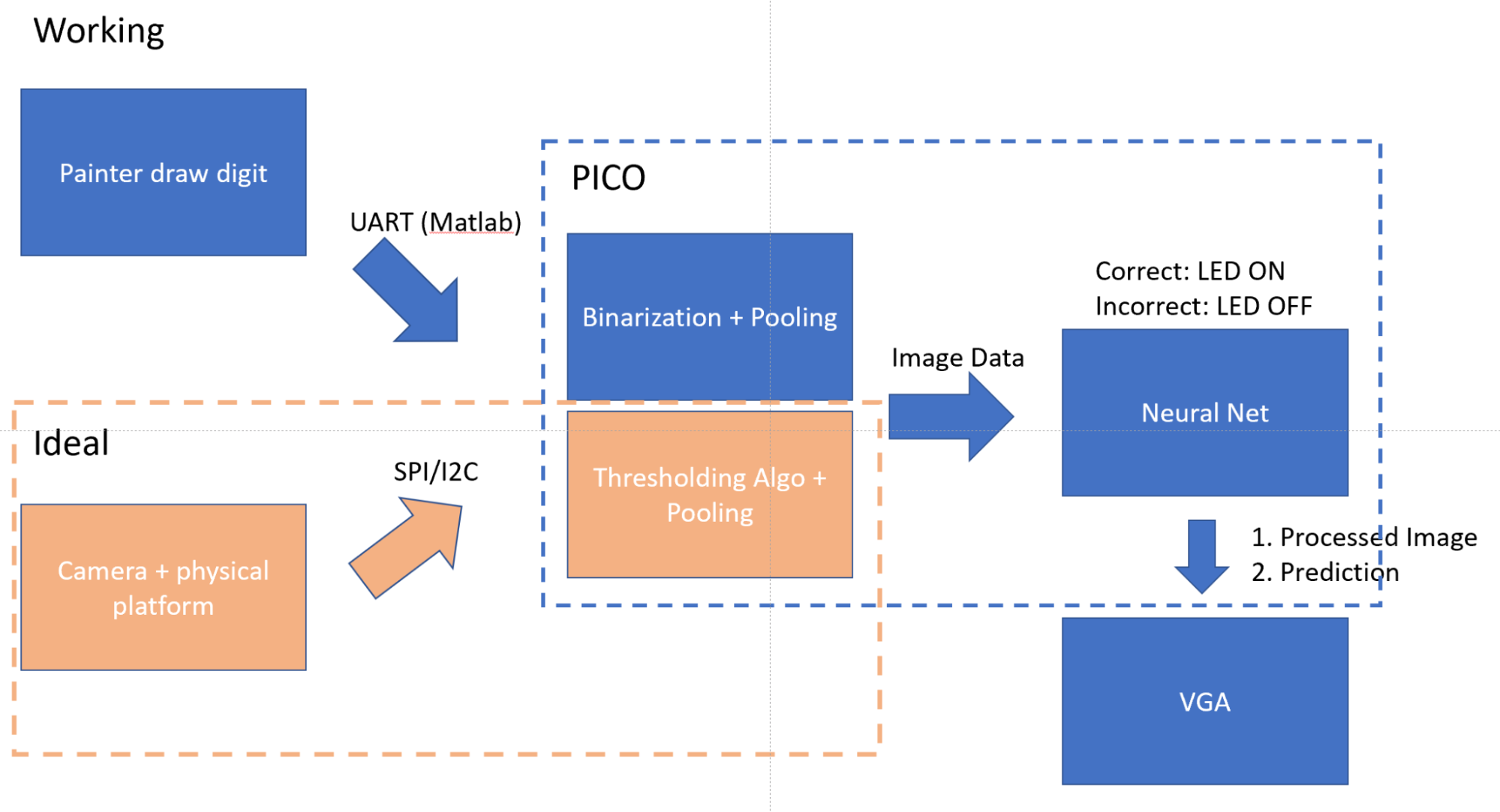
Without knowledge of the exact underlying technology, we made an educated guess that the system operated on a camera recognition system and decided to recreate it. We wanted to build a minimal viable system with a PICO running a machine learning algorithm that parses the camera information to perform digit recognition and sends the processed information and prediction to the VGA for display of results. Figure 1 is a diagram of the overall infrastructure, including the working version and ideal scenario.
Figure 1. System Infrastructure Diagram
The ideal approach implements a camera peripheral which is probed by the PICO to take a picture. The image data is transmitted via SPI or I2C to the PICO. We binarize the image data with a thresholding algorithm to combat external environmental variables such as lighting and pool the image to dimensions to fit our neural network model. The network is pre-trained with Matlab to recognize binarized 20 by 20 digit images. The input image and prediction is then drawn onto the VGA for display of results and a correct prediction will light up an LED that symbolizes the opening of a gate.
Unfortunately, we couldn’t get the camera to work so we pivoted to an alternative to showcase the potential results. Instead of feeding camera information to the PICO. We hooked up an UART channel that streams 256-color bitmaps created by the paint app to replace an actual person writing on a platform being captured by the camera. The thresholding algorithm is replaced with a more rudimentary cutoff algorithm since the input environment is more fixed.
We will still talk about our understanding and findings in getting the camera to work in the following sections.
Figure 2. Paint App
Mathematical Background
The main mathematical element to this project is the deep learning neural network algorithm that is implemented on the PICO. There are actually many algorithms that could be used for digit recognition from K-Nearest Neighbors to Multilayer Convolutional Neural Networks. KNN could potentially have low accuracy (low 90s if lucky) depending on the dataset used for training. On the other hand, complicated convolutional neural networks require too much memory (i.e. training dataset for KNN has the same problem) for the PICO to handle. We ended up settling with something in between, which is a multilayer perceptron model with 3 layers (i.e. input layer, hidden layer, output layer). This still pushed the PICO stack memory to its limits which will be discussed later.
Multilayer Perceptron Model
The layers of the network are 400 -> 25 -> 10 for the input layer, hidden layer and output layer, respectively. The input 400 is for a 20 by 20 image array, each value representing the value of a pixel (i.e. this is binarized). The middle layer values are the linear combination sum of the input values and the pre-trained weights.
The linear combination value of each node is passed through an activation function to introduce non-linearity before going to the next layer. The activation function we chose for this model is the sigmoid function Figure 3 which is
. By passing the value through the sigmoid function, we are able to have a more definitive value for the influence of a perceptron. This helps with the prediction of the neural network.
The last output layer has 10 perceptrons representing the 10 different digits (i.e. 0-9). The output perceptron that has the largest value is chosen as the prediction. It is easy to understand the meaning behind the input layer and the output layer, yet the hidden layer often lacks some intuitive explanation. Figure 4 is a snippet of deep learning video on Youtube from 3Blue1Brown that provides a reasonable visual insight behind the hidden layer. Essentially, the hidden layer selects pixels to form strokes that compose a digit. The pixels are the basic building block, and the hidden layer contains these intermediary blocks that form a digit.
Figure 3. Neural Network Model
Figure 4. Hidden Layer Intuition [# 3blue1brown reference]
Dataset & Training
Our dataset contains 5000 samples with 500 of each digit. The data originally came in some type of float representation so we made use of the thresholding algorithm to binarize the dataset. We used the dataset to train the weights via back propagation with Matlab. We will hold from discussing too in depth on the derivation of backpropagation. Essentially, backpropagation identifies which pathway (i.e. weights) in a neural network is more influential in the final prediction and updates all the weights to arrive at the desired prediction [8]. This is done by computing the partial derivative of the loss function with respect to all the weights.
3. Program/Hardware Design
Hardware Description
This lab involves three major parts in hardware, one is the OV2640 camera circuit (replaced with Matlab communication via UART), another one is the LED and the last one is the VGA. The below Figure illustrates the overall hardware connection between the RP2040, the VGA monitor, and the OV2640 camera. We were able to get the camera working but since it wasn’t used in the final infrastructure, we reconfigured the GPIO pins for I2C to UART.
Figure 5. Overall Setup
Camera Setup
Our camera is equipped with a 2-megapixel CMOS OV2640 image sensor. It supports RAW, YUV, RGB, and JPEG format outputs; also supports UXGA, SVGA, VGA, QVGA, CIF, and QCIF resolutions.
Figure 6. Camera board
The camera contains two interfaces, I2C for the sensor configuration, SPI for camera commands and data stream, handles the complex memory and user interface hardware timing.
Figure 7. Camera Block Diagram
Figure 8 shows the camera board pinouts, unlike the Arduino, Pi Pico has limited GPIOs but we still found a way to make connections, as the figure 9 shows below.
Figure 8. Camera Module Pinouts
Figure 9. Pin Mapping
Then we following the table above to complete the connections, as the figure shows below.
Figure 10. Connection with Pico
Figure 11. Camera Working
LED Setup
We hooked up an LED to GP15. The purpose of this is to use LED as an indicator, if the handwriting prediction is correct, then the LED will light up, no light otherwise. First we initialize the LED by set the GPIO #15 to output, and pull it to logic zero.
Figure 12. LED Initialization
Then we have a thread called protothread_blink, which monitors the plate_flag, and set the GPIO to logic one if the flag is true.
Figure 13. LED thread
UART
The Pi Pico have two UARTs, one we used (UART_0) for serial command input and output (GP0 and GP1), the other one (UART_1) is on GP8(TX) and GP9(RX), which we use it for upload bitmap image data. We initialize the UART_1 in the main function with the 115200 baud rate. During our test and debug, we found there is a consistency issue when deal with two UARTs. When we send data via the UART_1 and at the same time we read the UART_0, sometimes it works while sometimes it does not. We still cannot resolve this issue.
Figure 14. UART_1 setup
Paint App
Matlab allows for an easy setup of UART connection by calling the serial port function and specifying the channel and baud rate (i.e. matching the PICO). Writing and reading can be carried out after the port is established.
We specify the canvas dimensions via image properties on the paint application. In this case, our dimensions are 1800x1200 pixels. The bitmap is split vertically down the middle to separate the two digits (i.e. this is a constraint imposed on the user) and pooling is done to downsize the image into a 20 by 20 pixel bitmap to feed into the input layer of the neural net. The pooling algorithm we used is maximization pooling, meaning the pooled value is the maximize value of all pixels in the pool. Figure 15 show the raw bitmap from paint, after splitting, and after pooling. All of this is done on a local matlab script.
Figure 15. Painter properties, raw image, downsize image, pooling image
PICO
Functionality
In terms of work distribution on the PICO, we have core 1 cycling through three threads, one for turning on the LED, one for drawing on the VGA, one for serial user interaction. Core 0 handles all rest in one main loop, from UART data retrieval to neural network prediction.
Figure 16. Loop structure
In the main loop of core 0 on the PICO, we set up a loop structure to listen for the signal sent from the laptop running the matlab script. The data is stored in an array and there is a counter used to keep track of the amount of data received. When all 400 bytes are received, we call the feedforward function, which implements the neural network to make the digit prediction. The feedforward function is composed of a series of function calls (as mentioned in the mathematical background section ) that takes the input data and makes the prediction. Each step of the network is modularize