Kinetic molecular theory with particles

ECE 5730: Kinetic Molecular Theory with Particles on a RP2040
Demonstration Video
Objective
The purpose of this lab is to use the RP2040, DAC, and VGA to create a kinetic molecular theory physics simulation.
Introduction
The boids lab earlier this semester inspired us to understand other natural phenomena, so naturally we began to research different physics theorems. Due to the nature of the boids lab, we realized we could create an ideal gas law simulation that followed kinetic molecular theory. In order to verify the simulation was working as physics would expect, we implemented a representation of Boyle's law and displayed the kinetic energy average of the particles.
High Level Design
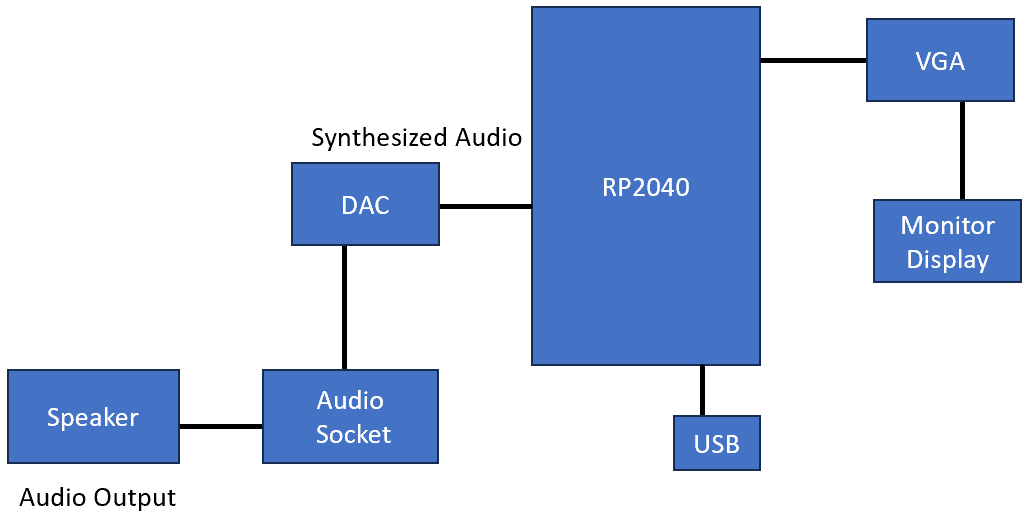
Figure 1: Higher Level Block Diagram
Boids Algorithm Background
Using different portions of the boids pseudocode from the
4760/5730 Boids Algorithm page
we were able to implement particle like behavior. Below are segments of the code that we found useful when simulating our particle movement.
Within our code the main focus was on the boid algorithm's use of visual range, speed limit, and updating of position.
Ideal Gas Law Background
Our particle model is based on the five postulates of kinetic molecular theory: (1) Gas particles move linearly unless a the particle collides with another particle or a wall (2) volume between particles is negligible because the free space between them is large (3) the particles collisions are elastic, so no kinetic energy is lost during collisions (4) there is no forces of attraction and repulsion between particles (5) the particles' average kinetic energy is proportional to temperature. Thus, for a group of particles average kinetic energy should remain constant in the model which gives us that KEavg= 0.5*m*vrms^2, where vrms is the root mean square velocity and m is the mass of the particle. Furthermore, using KEavg based on temperature we could directly relate our temperature to the particles' velocities such that vrms = sqrt(3RT/m). These postulates provide us with the ideal gas law PV = nRT, where P is pressure, V is volume, n is number of moles of a particle, R is the universal gas constant, and T is the temperature.
In relation to collision in our model, initially ran the program assuming the collisions would result in the particles just moving at the velocity of those reaching it, but the downfall of this method was not every collision was based on the particles' centers of mass. Based on this relationship a collision method had to be put in place. Using this new method and increasing visual range slightly we were able to create a more accurate collision model for the particles that kept our initial particle velocities consistent to what we expected.
Another component of ideal gas law we implemented in our simulation was Boyle's law. According to Boyle's law pressure and volume are inversely related and thus P is proportional to 1/V. In order to make sure that our program was acting in this manner we assumed temperature would be a constant that the user could change from Putty. Through the implementation of calculating Boyle's law at different temperatures, we had a theoretical check for our simulation's pressure vs. volume relationship.
An unexpected outcome of changing the temperature in this manner provided us with different isothermal graphs as derived in thermodynamics. Since the temperature was constant, change in temperature was zero and pressure vs. volume graph acted as one would expect isothermal graphs to act at different temperatures. In isothermal graphs as the temperature is increased energy within the system is increased, such a phenomenon was seen in our simulation as temperature was increased it had a direct impact on the kinetic energy average in our model.
Collision
In our collision simulation, we have the assumption that all particles have the same mass and the same velocity. Therefore, the collision model can be largely simplified. However, we cannot oversimplify the model. In our first model, we assumed that each particle has an infinite small volume and force field, so when two particles collide, we simply swap their moving direction. This made no difference between the non-colliding model.
Therefore, we introduced the second model: We assumed each particle had a specific volume. To implement this concept, we can translate it to: we perform collision of these two particles if their distance is within twice their radius.
Figure 10: collision illustration
The left picture shows the collision of two particles with the conservation of momentum. We can convert it to the right one for better understanding. Because the particle mass and the velocities are the same, we only need to consider the direction after the collision. Thus, the surface of the right picture circle serves as a mirror. Therefore, the collision can be modeled as follows:
Figure 11: collision_formula
Where vector u is the normalized vector that points from the center of the circle to reflecting point and 2(v u) u serves as the speed difference that v needs to change which is perpendicular to the surface of the circle. This equation can simulate the mirror reflection without too much computation cost and implementation complexity.
Hardware/Software Tradeoffs
There is no trade-off between hardware and software. They provide different functionalities in this project. Hardware provides DAC, Putty connections, and VGA output while software provides the simulation algorithm, system control and hardware resource manipulations. They cannot replace each other in any manner.
Program/Hardware Design
Our main objective was to adapt the boids code such that the particles collided like gas particles. From there we adapted the code so the user could input different amounts for the volume and see the different results of pressure (hitting rate per second) versus time. After getting a working model of the constant volume, we modified it by integrating a synthesized beep. When the beep was working correctly, we adjusted the code to beep every time a particle hit the wall of its volume. Once we had developed a constant volume, we made a simulation to develop pressure versus volume graphs at varying temperatures (chosen by the user). To verify that our pressure versus volume graph was behaving as expected, we plotted Boyle's law. Finally, we added a constant pressure graph so the user could see how kinetic energy would need to decrease if volume decreased at a constant pressure for varying temperatures. To verify that this was working correctly we found what the pressure should be based on the chosen temperature and plotted the result.
RP2040 Program Design
Our software architecture and computational power distribution
Core1 (main computation)
Particle simulation
Core2 (miscellaneous)
Particle simulation
Pressure calculation
Graph plotting
Serial input output
Our design principle is an incremental design. We complete each functionality by gradually adding features on it and making sure it works within our expectation every time. This is one of the most efficient ways to build up a complex system and we can narrow down the place that is most likely to produce bugs. Every time a feature is created, we would set up several hand-crafted unit tests to ensure the basic functionality. The methodology helps a lot even when the project scale grows up. More specifically and practically, we made the program highly modularized, in which we separated each functionality into several functions and made sure each function will not be too long to read or debug. Moreover, we try to keep everything as function calls instead of macro because the function can make a good isolation for variable names and take the advantage of C's type checking. There should be little or no drawback with modern compiler architecture. Functions can be inlined and therefore can have the same performance with macro which puts the program at risk by modifying the program in compile time.
Main Functions Explanation
Move_particles()
Figure 9: Move_particles() pseudocode.
All particles are stored in global variables and therefore can be accessed by every function, but this slightly decreases the safety of the program.
For each two particles, if they are both in each other's visual range, then a collision happens. The collision is explained in the physics section. The drawing part is relatively simple: for each frame, the previous positions will be erased, the position will be updated, and the new position will be printed (if the position is inside the bound).
This is the core computation in our project. If we do not perform the collision the time complexity of this function will be O(N), while our version of collision algorithm complexity is O(N^2) which is much higher and became the bottleneck. of the whole simulation. However, collisions are essential because we need to increase the 'chaos' of our system.
When the volume was changed, the moving wall generated a wavefront which made the measurement fluctuate and gave an imprecise measurement of collisions especially when the kinetic energy was at a lower state. Therefore, we still need collisions to increase the entropy even though, logically, the pressure will be measured the same in a long-term experiment.
According to the experimental result, the collision actually helps a lot. The wave-like moving particles will be eliminated in a short time (in 3-4 wave period) and quickly make the measured pressure converge to the ideal line. This is obvious when the volume is adjusted in a short period of time.
Beeping Sound Generator
The sound is generated by Direct Digital Synthesis Algorithm (DDS). The target sine wave will be incrementally generated with the timer interrupt callback. When a particle hits the wall, a swoop sound will be generated once. While the original sound is synthesized every 25 us, we change the frequenc