Interactive lightsaber

ECE 4760 Final Project:
The Interactive Lightsaber
Our project is a 24-bit RGB LED illuminated lightsaber that reacts to surrounding sound and
detects vowels.
Demo Video
Introduction
In Star Wars, each character has a fixed lightsaber color. Despite being two big Star Wars fans, we
wanted to change the fixed notion of lightsabers by creating one that would enable its users to have a lightsaber
that could be more than one color. So, using a microphone, RP2040, and an addressable LED strip, we created an
interactive lightsaber that changes based on audio input.
The first mode, disco mode, changes the color of the lightsaber based on the frequency and
intensity content of the surrounding sound. This was done through an FFT to gather frequency and intensity, which
were then mapped to HSV, where hue was determined based on the frequency and intensity configured the saturation
and value. Later, HSV was converted to RGB to be displayed on the lightsaber.
The second mode, vowel detection mode, changes the color of the lightsaber to red if the user says
"EE" and to blue if the user says "AH." This was done through the use of cepstral analysis,
which involves computing the FFT of the log-power spectrum, lowpassing, and achieving a smoothed power spectrum
through an inverse. This enables extracting the formant frequencies of the input sound, which we then compare with
the formant frequencies with EE and AH to determine if there is a match.
High Level Design
Rationale of Our Project:
The original vision of our project was to build an interactive lightsaber with two modes: Disco
mode and Character mode. Disco Mode changes the color of the lightsaber based on the surrounding sound frequency
and loudness. This mode was implemented in the final design. Character mode, on the other hand, changes the color
of the lightsaber to the specified character's lightsaber color. For example, saying "Darth Vader"
would change the lightsaber's color to red. However, this mode was too ambitious for a 5-week project;
therefore, we decided to create a more achievable "vowel recognition mode" instead, which changes the
color of the lightsaber based on the user saying EE or AH.
Disco Mode:
For this mode, we want the lightsaber to change color based on the input from the microphone. To do
so, we would need a function that takes in the frequency and intensity content of the surrounding sound and
converts it to an LED color.
We decided that the input frequency to the LED function should be the most intense frequency in the
surrounding sound, and the input intensity to the function should be the intensity of the most apparent frequency.
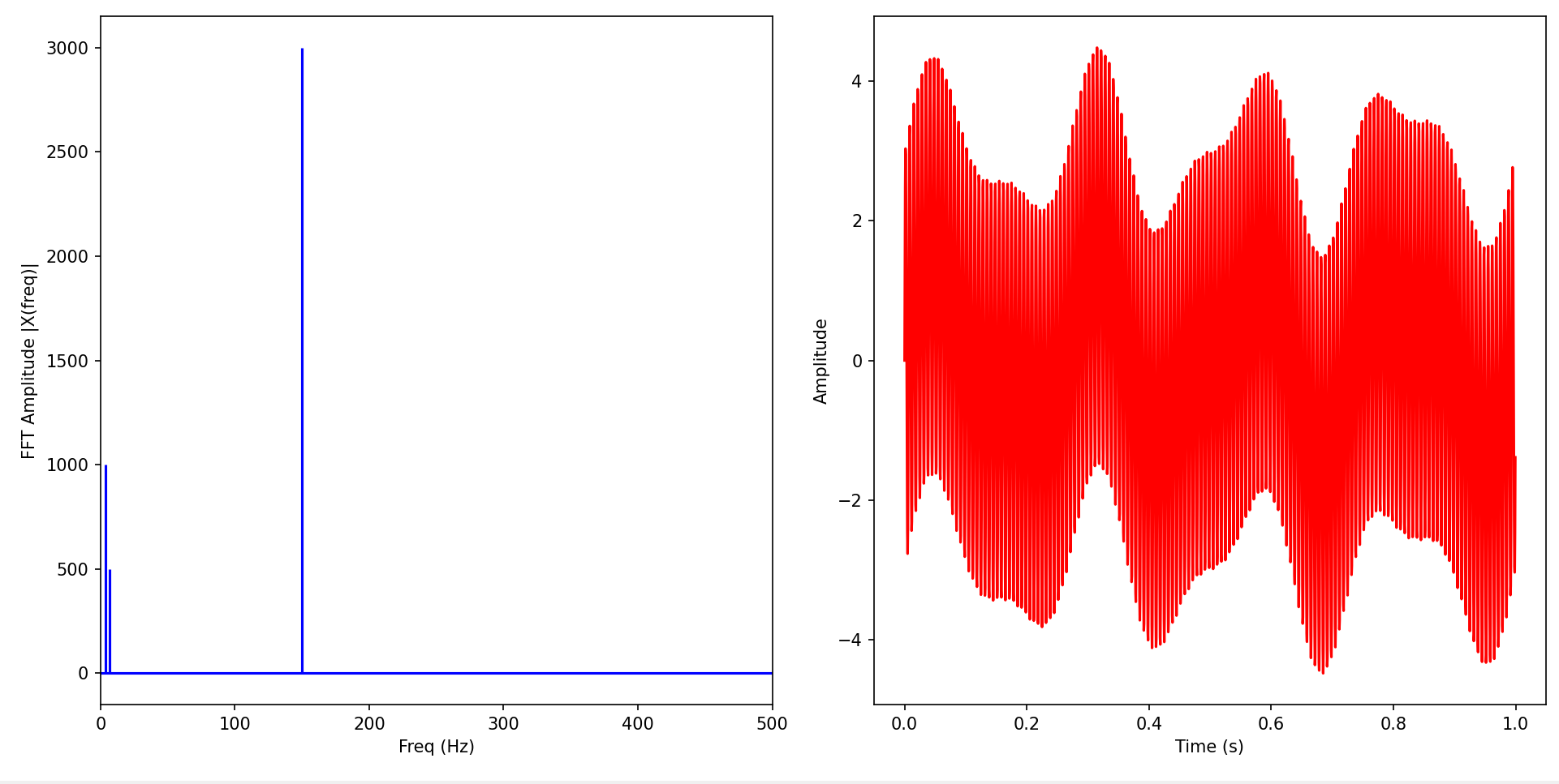
The simplest method to find such frequency and intensity is using an FFT. The figure below illustrates a random
signal and its FFT.
Figure 1.
Random signal (on the right) and it’s FFT (on the left)
In this example, the most apparent frequency is at 150 Hz with an intensity of 3,000. This is
clearly visible in the FFT. Therefore, through this method, we can easily extract the maximum intensity and
frequency of the signal.
After finding the frequency and intensity content of the input signal, we wanted to convert these
to RGB in a simple, linear function. However, RGB has three distinct color components, making it difficult to map
from frequency and intensity to color. Consequently, rather than converting it directly to RGB, we decided to
convert frequency and intensity to HSV first and then convert HSV to RGB. HSV also has three components: hue,
saturation, and value. Hue ranges from 0 to 360 degrees, and saturation and value range from 0 to 1. The image
below shows how each parameter varies the resulting color:
Figure 2.
Illustration of how hue, value, and saturation changes output color. Source: Appendix B, 9
As seen by the figure above, the hue controls the base color, while intensity and saturation
control the purity and brightness, respectively. As a result, unlike RGB where three distinct channels control the
color, in HSV, only the hue impacts the base color, so we can easily create a linear mapping from frequency to
hue. Then, we can map intensity to saturation and value. As a result, given a frequency (0 to 1,500 Hz), we scale
the frequency to the hue spectrum (from 0 to 360 degrees), and given an intensity (0 to max_intensity), we scale
the intensity to the saturation and value spectrum (0 to 1). The diagram below illustrates this
transformation:
Figure 3.
Transformation of input frequency and intensity to HSV
After the frequency and intensity is linearly mapped to HSV, the last step of the disco mode is to
convert HSV to RGB, which is a commonly used formula illustrated below:
Figure 4.
Formula for HSV to RGB. Source: Appendix B, 10
To summarize this process, we first obtain the most intense frequency and its intensity using an
FFT. Then, we linearly map the frequency and intensity to HSV by mapping frequency to hue and intensity to
saturation and value. Finally, since the LED accepts RGB, we convert HSV to RGB.
Vowel Recognition Mode:
In order to achieve vowel recognition for recognizing the difference between EE and AH sounds (or
any other vowel), we need to extract a set of frequencies called “formant frequencies,” which
represent the acoustic resonance at particular frequencies. This method works perfectly for our vowel recognition
functionality because each vowel sound has a set of unique formant frequencies, illustrated in the table
below:
Figure 5.
Set of formant frequencies for several vowels. Source: Appendix B, 11
For our case, we are interested in the frequencies of the EE and AH sounds. According to the source
corpus (see Appendix B, 12), the table below shows the expected formant frequencies of the EE and AH
sounds:
Table of Formant Frequencies for EE and AH sounds
F1
F2
F3
EE
300 Hz
2,400 Hz
3,000 Hz
AH
700 Hz
1,100 Hz
2,400 Hz
As a result, if we can successfully extract the input signal's formant frequencies, we can
easily compare the extracted frequencies with the expected ones of EE and AH and pick the one that matches it the
best.
To classify a sound as EE or AH, first plan to use a fixed range to see if frequencies fall in a
given range. Then, we plan to use a fixed range and L1 distance as it is computationally light and an easy way to
compare how close a set of three formant frequencies corresponds to the set of expected ones. The formula below
shows how L1 computation is done:
L1 Distance = |x

- x

| + |y

- y

| + |z

- z

An important note about formant frequencies is how much they differ from person to person
(especially male to female). As a result, we plan to make the classification somewhat loose to account for
frequency changes depending on the person. Loose classification may cause misclassification; we plan to test this
after completing the system.
As mentioned earlier, the success of this functionality relies heavily on extracting the formant
frequencies in an accurate and timely manner. To do so, we plan to use a method named cepstral analysis, which
involves six steps:
Pre-emphasis: Boosts the higher frequency components of the input.
Window: Apply cos window to add periodicity to input.
Compute log power spectrum by taking the FFT, taking the magnitude of the FFT, and taking the
log2 of the magnitude.
Convert to cepstrum: Take the FFT of the log power spectrum.
Truncate/lowpass: Smoothens final output and gets rid of fast changes in the cepstrum.
Convert back to the power spectrum by taking the inverse FFT.
The figures below demonstrate the cepstrum and the smoothed power spectrum for a random
signal:
Figure 6.
Cepstrum of a random signal
Figure 7.
Smoothed power spectrum of a random signal
As seen from the above graphs, the cepstrum appears sporadic and hard to analyze, while the
smoothed power spectrum appears less daunting and visually more appealing, which is the primary purpose of
creating this smoothed spectrum. The x-axis in both graphs corresponds to the sample. For example, the above
graphs have 128 samples, and if they can detect frequencies from 0 to 4,000 Hz, each sample would correspond to a
4,000 Hz / 128 = 31.25 Hz window. Thus, if a peak was detected at sample 10, there is a formant frequency of
around 312.5 Hz. Thus, to extract the three formant frequencies, we would find three peaks and which frequency
window they correspond to.
To summarize the entire vowel recognition process, we first use the six steps above to get the
smoothed power spectrum of the signal. Then, we pick the first three peaks above a certain noise level determined
based on experiments and extract the frequencies of these peaks (which correspond to the formant frequencies).
Then, we compute the L1 distances of these frequencies with the expected formant frequencies of EE and AH sounds.
If the distance meets the criteria of the classification, then it is recognized as an EE or AH sound.
Software and Hardware Trade Offs:
The two leading hardware trade-offs are the microphone quality and the quality of the onboard ADC
on the RP2040. As the microphone gets more expensive, the quality of the acquired input signal improves, enhancing
the output of the FFT and the power spectrum. However, when we ran the example FFT code, the microphone from the
lab did a sufficient job of displaying the correct FFT, so we decided to use the cheaper microphone. Another
hardware trade-off is the onboard ADC, which impacts how frequently we can sample data. Due to the spac