DJ 2040

Introduction
High Level Design
Software Design
Hardware Design
Results
Conclusion
Appendices
References
DJ 2040: Final Project for Cornell ECE 4760
Jacob Tamor, Madeleine Lee, Michael Awad
Section 1: Introduction
The DJ 2040 allows users to tune audio input in the frequency domain and visualize the sound on a display!
This project was inspired by recording studios and the ability to manipulate audio inputs.
We process the inputted audio through an ADC channel, apply an FFT to it, apply a filter to the FFT,
and then compute the inverse FFT of the filtered frequency-domain signal. The results of the inverse FFT
are written to the DAC and outputted through a speaker. This is all done in real-time. To filter the signal,
two potentiometers are used. The first potentiometer tunes the lower frequencies, and the second potentiometer
tunes the higher frequencies. This gives the user the control to alter the sound of a song in a way that
mimics a DJ board. Finally, the tuned audio in the time domain along with the levels of the potentiometers
are outputted to the VGA display, providing a visual user interface.
Section 2: High Level Design
Because any music or audio is composed of many different pure sine wave frequencies added together, audio can be represented as the sum of many, if not infinitely many, sine waves. Thus, in constructing sound in this way, the frequency spectrum can be viewed as being comprised of many frequencies at different amplitudes. The fact that sound can be decomposed into separate frequencies is advantageous when attempting to modify the sound according to different frequency ranges.
Our design utilizes FFTs and IFFTs to convert data from the time domain to the frequency domain (FFT) and back (IFFT). In the time domain, the main manipulations that can be performed on sound are volume, which corresponds to the amplitude of the voltages being outputted, and playback speed, which corresponds to how quickly we output samples. However, to change the volume of sound within a specific frequency range (much like the bass, mid, and high knobs on a common DJ board or music synthesizer), the use of frequency filters or amplifiers is required. This computation could be done using filters and convolutions in the time domain, but it is much easier to achieve this same behavior by running FFTs on the sound frames and performing element-wise multiplication in the frequency domain, where these multiplications are chosen to scale the magnitude of the sound at the given frequency.
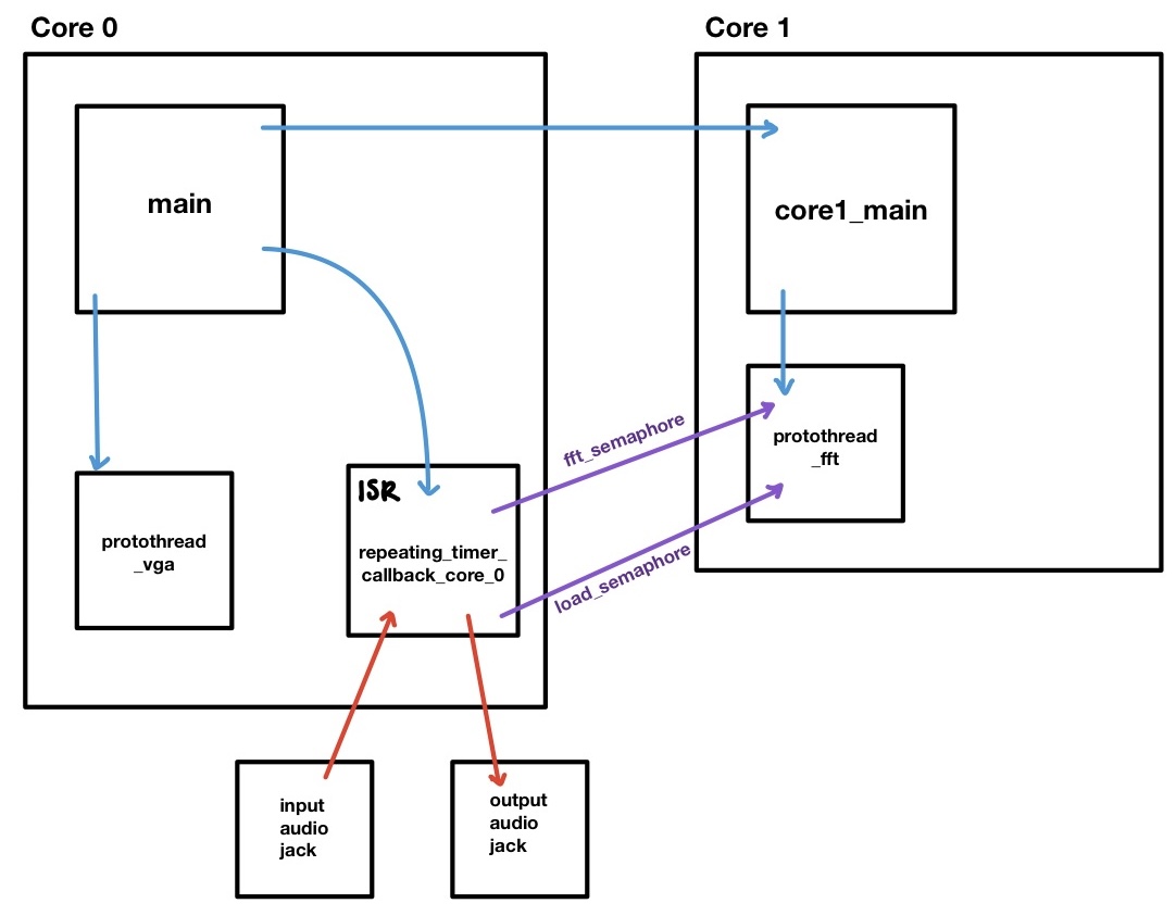
In terms of implementation, our design uses both cores, two protothreads, an interrupt service routine triggered by a repeating timer, and two semaphores to synchronize the ISR and the FFT computation thread. The figure below shows the interactions between all of these software components.
Figure 1: High Level Software Diagram
We decided to put the protothread_fft as the sole thread on Core 1 because it is responsible for computing both an FFT and an inverse FFT for each sound frame (1024 samples). All of these computations must occur during the time that it takes the ISR to output the previous frame. The ISR runs every 80 microseconds, so this time can be calculated as follows:
1024 samples * 80us/sample = 81920us =
81.920ms of maximum computation time allowed per frame
This is plenty of time for the FFT thread to finish its calculations. However, because of the timing dependencies between the ISR and the FFT thread, we did not want protothread_fft to share its core with any other thread. We also separated the ISR and protothread_fft into different cores so that they could run fully parallel to each other, allowing protothread_fft the full 81.920ms of computation time.
In the same vein, we decided to run the protothread_vga on Core 0 with the ISR because it is less computationally expensive, less critical to the functionality of our design, and less time-sensitive than protothread_fft.
Section 3: Software Design
3.1 Audio Processing
The audio processing techniques used can be structured in three different stages: audio input reading, frequency domain manipulation, and audio output. Analog voltage inputs into the RP2040 and outputs to the speaker are both done inside of the ISR running at 12.5 kHz, allowing for strict synchronization with audio sampling and output.
The reading of the audio output is done with ADC channel 0. With the DC-biased voltage that comes out of the audio connector and into the ADC channel, the program can directly read the ADC channel and extract the analog voltages that correspond to the sound being streamed in. The numbers that directly come from the channel will not be the actual values of voltage that is seen at the ADC channel input but instead represent the voltage level with respect to the ADC’s resolution and the reference voltage that the ADC uses. However, because all these numbers are in the same proportion to the real analog voltage values, it is unnecessary to convert the values to their analog voltages when computing any of the audio processing algorithms. As the audio is streamed in, 1024 samples are taken from the ADC before running an FFT on that frame. Once there is data for the sound in the frequency domain, the frequency manipulation by virtue of the potentiometer knobs can take place.
Computations for audio control using the potentiometer knobs are done right before the IFFT is run on the audio frame. The inputs at the ADC channels that correspond to the potentiometer knobs see a voltage between 1 and 3 (which is explained further in the Hardware Design section), and thus in order to use these as scalars to the audio, they must be converted from the ADC units to their actual voltage values. Once the voltage values are calculated, the scalar to be used is that voltage minus one, allowing the audio control to range from zero to double the inputted volume. Right before running the IFFT, a loop goes through each value of the frequency spectrum and multiplies them by the scalar calculated from the current value of one of the ADC channels. One of the knobs controls the magnitude for frequencies below 400 Hz and the other controls frequencies above 400 Hz. After looping through the frequency spectrum and manipulating the magnitude for the target frequencies, the IFFT is run on the edited spectrum. The conversion of this frame back into the time domain gives us the analog voltages that should be outputted to the speaker at the same sampling rate it was received.
Outputting the sound to the external DAC requires configurations specific to the DAC, and also a bit more audio manipulation in order to make the sound a good volume for us to hear. In every instance of the ISR running, one value from the manipulated sound array is first multiplied by 2 (in order to increase the volume of the sound), cast to an integer from a fix15 value, and masked according to the configuration requirements for the DAC used. Once these operations are performed on the analog value, this number is written to the DAC using SPI. One of the DAC’s voltage outputs is directly connected to both ends of the output audio connector, which is then connected to an audio cable for a speaker to output the received sound.
3.2 Software Implementation
The primary functionality of our project is the audio processing component. In our software, this consists of the ISR and the FFT protothread (protothread_fft). These two functions communicate with each other through semaphores, which ensures that each step of the process is synchronized properly while allowing the ISR and protothread to run in parallel. The basic functions of both components as well as their communication are described in the pseudocode in Figure 2 below.
Figure 2: Pseudocode for ISR and protothread_fft
At a high level, the ISR is responsible for the input and output of audio data from the RP2040, and protothread_fft is responsible for all of the audio processing that occurs in software. As shown in Figure 2, the ISR collects inputs, the protothread_fft performs the audio processing computations described in section 3.1 above, and the ISR takes the resulting data and outputs it to the DAC.
It is important to note that the inputting and outputting within the ISR occur sample by sample. That is, for each run of the ISR, one sample is loaded into fft_buff_r and one sample is outputted to the DAC from interrupt_fft_array. However, the other processes such as copying the samples and signaling the semaphores only occur once every frame (1024 samples). This ensures that the audio samples are being collected and outputted at the same rate (12.5kHz).
In addition to the ISR and the protothread_fft, we use different arrays for each stage of audio processing. This allows us to perform each stage in parallel with each other which in turn helps ensure that we are able to do all of the computation while still inputting and outputting at a consistent 12.5kHz. That is, we are able to both take in audio samples, output audio samples and perform computations on audio samples concurrently. We used the memcpy C function to reliably copy data between arrays without pointer dependencies.
Array
Purpose / Stage
fft_buff_r / fft_buff_i
Audio input- the input audio is loaded into the fft_buff_r array and the fft_buff_i array is initialized to 0 since the voltages in the time domain do not have any imaginary components.
fr / fi
Audio processing- all of the FFT, frequency domain manipulation, and IFFT computations are done with these arrays.
interrupt_fft_array
Audio output- after the audio processing stage is finished, the fr array is copied into this array which is then read by the ISR and outputted to the DAC.
Table 1: Audio Data Arrays
3.3 VGA Graphics
Figure 3: VGA Display
The VGA display was modeled after Professor Adams’ FFT to VGA display project, with the main difference being that we displayed the voltage amplitude of our s