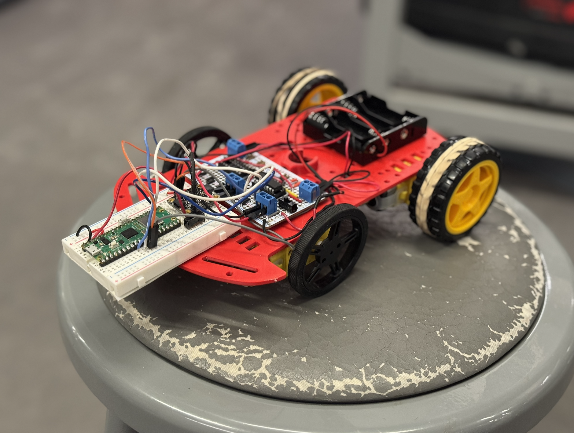
Autonomous Drawing Car

Final Report
Project Introduction
Project Sound Bite
An autonomous drawing car that turns mouse-drawn inputs displayed on a VGA GUI into real-world motion by wirelessly driving a robot car along digitally generated paths.
Figure:
Autonomous drawing car
Summary
What we did:
We built an autonomous drawing system using two Raspberry Pi Pico Ws that communicate over UDP. One Pico W interfaces with a PC, handling mouse input and VGA output to generate and display waypoints. These waypoints are transmitted wirelessly to a second Pico W mounted on a car. The car uses a 9-axis IMU to determine its orientation, computes PWM values, and drives its motors to reach each target point. The system supports two operating modes. In direct-follow mode, the car traces the path exactly as drawn. In optimized-route mode, the car calculates the shortest path through all points, improving efficiency while preserving the overall flow.
Why we did it:
One group member admired a previous year's drawing robot, and we share an interest in cars and Formula One. All group members work on a student project team that builds autonomous air systems, which motivated us to explore similar concepts on the ground. We wanted to combine creative expression with autonomous vehicle concepts like navigation, state estimation, and control. The project required us to work through autonomous navigation, reliable wireless communication, and real-time control while building something engaging to watch and satisfying to tune.
High Level Design
Rationale and Sources
Our drawing and communication subsystems are based on reference designs and sample code from ECE 4760 course materials provided by Professors Bruce Land and Van Hunter Adams. For the drawing interface, we adapted Professor Land's USB Host HID and VGA graphics demonstrations for the Raspberry Pi Pico RP2040. These examples showed how to run USB mouse input, VGA output, and protothreads concurrently across both cores. We modified this structure to sample mouse position data, generate waypoints, and render the drawing in real time on a VGA display.
The VGA graphics framework and USB HID handling provided a stable foundation. The separation of USB tasks, VGA graphics, and event-handling logic informed our thread organization. We modified the example code to stream drawing coordinates rather than perform direct on-screen drawing, allowing the generated data to be reused as motion commands for the car.
For wireless communication between the two Pico Ws, we based our design on Professor Land's UDP data transfer examples using LWIP and protothreads. These examples demonstrated efficient, low-latency communication between Pico Ws on the same network. We adapted this approach to continuously transmit waypoint data from the PC-side Pico W to the car.
We also used reference material and sample code from Professor Hunter Adams. PWM generation for motor control was adapted from course examples demonstrating the RP2040's hardware PWM peripherals. Sensor interfacing and I2C communication patterns were informed by Professor Adams' sample code, which we extended to support our onboard sensors.
For orientation sensing, we combined these course references with an external driver for the BNO055 9-axis IMU. We adapted the BNO055 driver from the JRDPropulsion BNO055-RP2040-Library (
https://github.com/JRDPropulsion/BNO055-RP2040-Library/blob/main/src/BNO055.cpp
), converting it from C++ to C for use with the Pico SDK. The driver handled low-level device configuration and data acquisition, allowing us to focus on heading estimation and motor control rather than register-level setup.
Building on established course examples from both professors let us avoid reimplementing low-level drivers and focus on system integration, control logic, and overall behavior.
Background Math
Mathematical Background: Baseline Navigation
This section describes the mathematical model used for baseline robot navigation through a sequence of user-defined waypoints. The approach combines planar geometry, trigonometry, and simple threshold-based control to guide a differential-drive robot along straight-line segments between waypoints.
Coordinate System and Robot Pose
The robot operates in a two-dimensional Cartesian world frame. Its pose is represented as
\[
\mathbf{p} = (x, y, \theta),
\]
where \(x\) and \(y\) denote the robot's position and \(\theta\) is the robot's heading angle in radians, with \(\theta = 0\) aligned with the positive \(x\)-axis. Each waypoint is defined as a fixed target position
\[
\mathbf{w}_i = (x_i, y_i).
\]
Distance to a Waypoint
The straight-line distance from the robot to a target waypoint is computed using the Euclidean distance formula:
\[
d = \sqrt{(x_i - x)^2 + (y_i - y)^2}.
\]
This distance determines how long the robot drives forward after aligning its heading with the waypoint.
Angle to a Waypoint
The absolute direction from the robot to a waypoint in the world frame is computed using the two-argument arctangent function:
\[
\theta_{\text{target}} = \operatorname{atan2}(y_i - y,\; x_i - x).
\]
The use of \(\operatorname{atan2}\) ensures correct angle computation across all quadrants and avoids division-by-zero errors.
IMU Heading and Degree-to-Radian Conversion
The robot’s heading is measured by an onboard IMU as a yaw angle in degrees. For use in trigonometric calculations, this value is converted to radians:
\[
\theta = \theta_{\deg} \cdot \frac{\pi}{180}.
\]
Using radians ensures compatibility with standard math library functions.
Heading Error and Angle Normalization
The signed heading error between the robot’s current orientation and the desired waypoint direction is given by
\[
e_\theta = \theta_{\text{target}} - \theta.
\]
Because angular quantities are periodic, this error is normalized to the interval \([-\pi, \pi]\) to ensure the robot always turns along the shortest angular path:
\[
e_\theta \leftarrow
\begin{cases}
e_\theta - 2\pi, & e_\theta \ge \pi,\\
e_\theta + 2\pi, & e_\theta < -\pi,\\
e_\theta, & \text{otherwise}.
\end{cases}
\]
Angular Tolerance and Alignment
Perfect alignment is unnecessary and can cause oscillatory behavior. Instead, the robot is considered aligned when
\[
|e_\theta| < \theta_{\text{tol}},
\]
where \(\theta_{\text{tol}}\) is a predefined angular tolerance. This threshold improves robustness and reduces control chatter.
Differential-Drive Turning Logic
The robot uses differential drive to rotate in place by driving the left and right motors in opposite directions. The sign of the heading error determines the direction of rotation:
\[
\begin{cases}
e_\theta > 0 \;\Rightarrow\; \text{turn right},\\
e_\theta < 0 \;\Rightarrow\; \text{turn left}.
\end{cases}
\]
A constant-magnitude PWM signal is applied during turning, resulting in a bang-bang control strategy.
Distance-to-Time Conversion for Forward Motion
Once aligned, the robot drives forward for a duration proportional to the computed distance. Assuming a constant linear speed \(v\), the required travel time is
\[
t = \frac{d}{v}.
\]
This time is converted into milliseconds or microseconds for implementation. The approach is open-loop, meaning the robot does not continuously measure distance during motion.
PWM Scaling and Saturation
Motor commands are implemented using pulse-width modulation (PWM). Commands are constrained to hardware-safe limits:
\[
0 \le \mathrm{PWM} \le \mathrm{PWM}_{\max}.
\]
A signed PWM convention encodes both direction and magnitude, ensuring safe and consistent motor control.
Baseline Navigation Assumptions
The baseline navigation model assumes:
Motion occurs on a flat 2D plane.
IMU heading measurements are sufficiently accurate.
Forward speed is approximately constant at a fixed PWM level.
Wheel slip and external disturbances are minimal.
Mathematical Background: Optimized Path Planning
In addition to baseline waypoint following, an optional path optimization step is implemented to reduce total travel distance. This optimization operates on the set of waypoints before transmission to the robot and is independent of the low-level motion controller.
Problem Formulation
Given a starting position \(\mathbf{s}\) and a set of \(N\) waypoints
\[
\{\mathbf{w}_1, \mathbf{w}_2, \dots, \mathbf{w}_N\},
\]
the objective is to determine an ordering of the waypoints that minimizes the total path length
\[
L = \sum_{k=0}^{N-1} \left\lVert \mathbf{p}_{k+1} - \mathbf{p}_k \right\rVert,
\]
where \(\mathbf{p}_0 = \mathbf{s}\) and \(\mathbf{p}_{k}\) denotes the \(k\)-th waypoint in the chosen route. This problem is a variant of the Traveling Salesman Problem (TSP), which is NP-hard.
Nearest-Neighbor Heuristic
To construct an initial feasible route efficiently, a nearest-neighbor heuristic is used. Starting from the current position \(\mathbf{s}\), the algorithm repeatedly selects the closest unvisited waypoint:
\[
\mathbf{w}_{\text{next}} = \arg\min_{\mathbf{w}_i \in \mathcal{U}} \left\lVert \mathbf{w}_i - \mathbf{p}_{\text{current}} \right\rVert,
\]
where \(\mathcal{U}\) is the set of unvisited waypoints. This approach produces a valid route with low computational cost, though it is not guaranteed to be globally optimal.
2-Opt Local Improvement
To further reduce total path length, the route produced by the nearest-neighbor heuristic is refined using a 2-opt local optimization method. Two edges in the route,
\[
(A \rightarrow B) \quad \text{and} \quad (C \rightarrow D),
\]
are replaced with
\[