Audio spatializer
This webpage is the final report for our final project in ECE 4760 Microcontrollers Fall 2022 and contains a detailed write-up about our project motivation, planning, design, implementation, results, along with things we learned and solutions to problems we encountered along the way. We also include solutions to problems that we could not add due to time/space constraints, and explanations for how and why they work, as well as ideas for future extensions of fe
- Suitable forB.Tech/B.E Embedded Systems students
- Build time4-6 weeks
- LevelAdvanced
- Available atAjvika Labs, Kakinada
About this project
Background
High Level Design
Hardware Design
Software Design
Results
Conclusions
Appendix
Audio Spatializer
Bianca Tseng, Crystal Shi, Rosie Wildermuth
This webpage is the final report for our final project in ECE 4760 Microcontrollers Fall 2022 and contains a detailed write-up about our project motivation, planning,
design, implementation, results, along with things we learned and solutions to problems we encountered along the way. We also include solutions
to problems that we could not add due to time/space constraints, and explanations for how and why they work, as well as ideas for future extensions of features that
could further improve the project.
Project Introduction
Our project is a real time audio spatializer that allows the user to adjust their aural experience by changing the perceived location and distance of the source of the audio they are playing.
In recent years, spatial audio has had a grip on video viewing platforms such as TikTok and YouTube, where viral videos will tell users to
“put on headphones for the full experience” and take them through an audio experience that makes them feel immersed in some sort of audioscape —
such as being in the middle of a conversation, getting a haircut at a barbershop (
The Virtual Barbershop
),
or scarily realistic simulations showing off 3D audio technology (
The Tucker Zone
).
We were fascinated by how convincing these effects were, and wanted to learn more about how they were implemented.
Further inspired by the concept of 8D audio, we wanted to explore ways to transform normal audio we listen to with our headphones and give it the same spatial effect.
8D audio is a type of audio effect typically used for music where, when wearing headphones, sounds seem to be coming from different locations in the room.
Usually, this effect is implemented on specific songs and heavily edited to cater to that specific song and make the user think that different parts of the song are coming
from different parts of the audioscape. We implemented an alternative to this, where instead of different parts of the song coming from different locations, the user could
adjust the perceived location of the song as a whole by dragging around a virtual, on-screen audio source. By simply putting on a pair of headphones, the user is immersed
into an aural landscape that is under their complete control, and can be applied to any song or audio they would like to hear.
The user is able to interface with a GUI to adjust the distance, angle, volume, and filtering of the audio they are inputting into the system in real time.
Background Information and Research
Our original project idea was to have a mostly stationary audio source, and to have a device that tracks the user’s head so that when they move their head,
the audio sounds like it is still coming from the same location. However, because of hardware and time constraints, we used a GUI to mimic the position of the
audio source relative to the head. We also realized that it would be very difficult to track head angle with the gyroscope and accelerometer as we originally planned.
This is because the gyroscope is prone to error accumulation over time, and unlike in lab 3, we would be unable to get good accelerometer readings to do complementary
angle calculation because our primary head movements would be side-to-side, which are very difficult to get readings from the accelerometer for. Thus, we switched to
using only the GUI to change the location of the audio, which worked a lot better than getting gyroscope readings and was also faster since we no longer needed to
calculate a complementary angle and head location based off of the sensor measurements. This improved processing speed and made our goal of real-time processing much
more feasible. Additionally, having a GUI greatly improved the user’s ability to interface with the program, as we were able to adjust a lot more parameters such as
precise distance, angle, location, volume, and whether the spatial filtering was on or off. It also made our design more modular as we now had another separate
component interfacing with our C program, and we were able to build, test, and debug these two programs separately. This helped in our design process and made it
easier for different group members to work on different parts of the project at the same time.
We spent a lot of time in the beginning reading papers and doing research about industry practices for making sound appear to be coming from specific directions
and distances. We found that most industry practices use Head-Related Transfer Functions (HRTFs), which define a frequency related transformation on the audio
that is dependent on the angle of the source to each ear in 3D space. This is because
audio signals are transformed by the external human ear structure, and this transformation differs depending on the angle of the source to the ear, as well as each
person’s individual ear shape and structure. These HRTFs are usually calculated experimentally by placing small microphones in the ears of a human or a
mannequin and recording the baseline impulse response of each ear after sampling an input from many different locations in 3D space. These samples are used to create
a database of HRTFs
which then can be applied to spatialize audio. We briefly entertained the possibility of obtaining HRTFs and using them for our transformation, but quickly realized
that the large size of each HRTF combined with the large number of HRTFs we would need to cover a wide range of spatial locations would be impossible given the memory
and processing constraints of our hardware. Thus, we decided to focus on azimuth (side to side, disregarding elevation changes) movement of audio sources, and
implemented other methods to achieve the spatial audio effect: amplitude difference, delay (phase difference), and low pass filtering.
High Level and Algorithmic Design
The goal of our program is to read audio input data, process it according to information about the location of the virtual audio source, then output the processed audio data in real time.
We designed the program flow and mathematical algorithms, as well as applied optimizations to our program to meet the time constraints of real-time processing.
Logical Structure
For our main program logic, we read an audio sample from the ADC into an input buffer and output a processed audio sample stored in an output buffer every 80 microseconds (12.5 kHz sampling frequency).
Concurrently to our input/output streaming, we also process the input audio signal to transform it into a spatialized output audio signal.
This guarantees that we are consistently reading the input audio without skipping or lagging, and that we are outputting samples at the same rate so we don’t pitch shift or cut off parts of the audio stream.
In the background, a serial thread polls and parses messages sent from the python gui about the audio source position, the volume, and left and right audio amplitudes,
and a vga thread updates the graphics on the VGA monitor to display left and right amplitudes and delays, graph the processed output from the DAC_output,
and graphs the frequency spectrum of the FFT and low pass filter results.
Amplitude Algorithm
The processing includes amplitude scaling, introducing a delay between the two channels, and a digital low pass filter through convolution, which we can do by performing the Tukey-Cooley Fast Fourier Transform (FFT) on the audio input samples.
When our samples are converted to the frequency domain, the convolution simply becomes element-wise multiplication, so we can perform the multiplication and then convert back to time domain through performing an IFFT.
Our IFFT operation uses the properties of FFT by scaling the conjugate of the FFT of the conjugate of the frequency domain signal.
Though this sounds complicated, it is actually faster to convert to frequency domain, multiply, and then convert back to time domain, rather than trying to do the calculations in the time domain.
We designed and implemented our own algorithms for the relative amplitude of the audio source to each ear based on angle and distance, the relative delay between the two ears,
and the cutoff frequency for our digital lowpass transfer function.
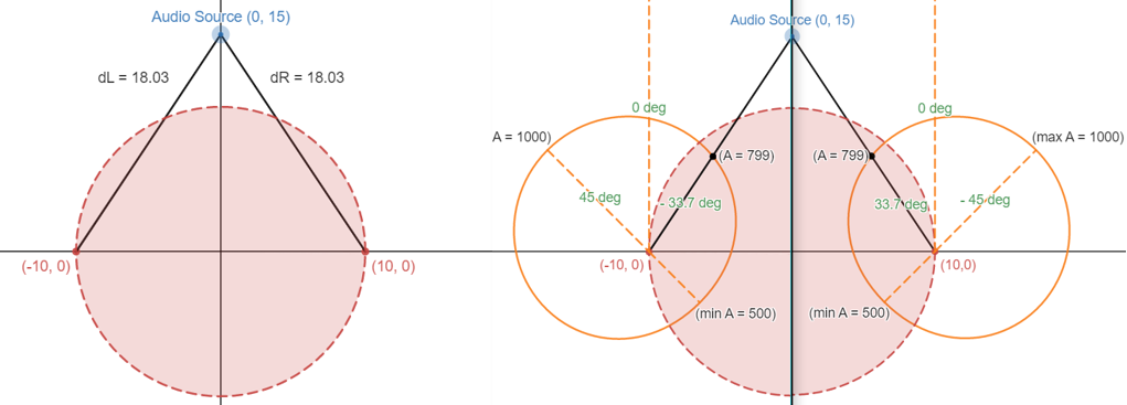
The angle-based amplitude calculation first scales the amplitude between 500 and 1000 based on the angle of the source to the ear.
We define 0 degrees to an ear the angle facing directly forward from a person's head, and increment degrees in the counterclockwise direction.
The left ear therefore has a maximum amplitude at 45 degrees, and the right ear at -45 degrees. This relationship is shown as the orange shapes in Figures 1 and 2 below,
with the radius representing the amplitude at that angle. We chose this model because we knew the shape of the external ear would attenuate sound more from certain angles,
and we also wanted amplitudes to be softer behind the head than in front.
The choice of cosine was intuitive to make the transition from minimum to maximum amplitude very smooth, as can be seen in the roundness of the diagrams
Technologies used
Hardware components
- IMU
- gyroscope
- accelerometer
- microphone
- DAC
- ADC
Software & tools
- Python
Project demo video
What you get
- Working project / hardware kit, tested before delivery
- Complete source code with explanation
- Project demo and guidance for your viva
- Project report, PPT and IEEE paper support (on request)
Related Embedded Systems projects

Gas Leakage Detector Using Arduino
A budget-friendly LPG gas leak detector built with an Arduino and MQ-5 gas sensor, triggering a buzzer and LED when unsafe gas levels are de...
View project
Simple Alarm System
A beginner-friendly home alarm with PIR motion sensing, keypad PIN entry, and separate entry/exit timing delays, built to be easy to expand.
View project
Ultrasonic Sensor Project with Arduino UNO Q
A beginner-friendly first Arduino UNO Q project: a servo-swept ultrasonic sensor that renders a live sweeping radar display in a web browser...
View project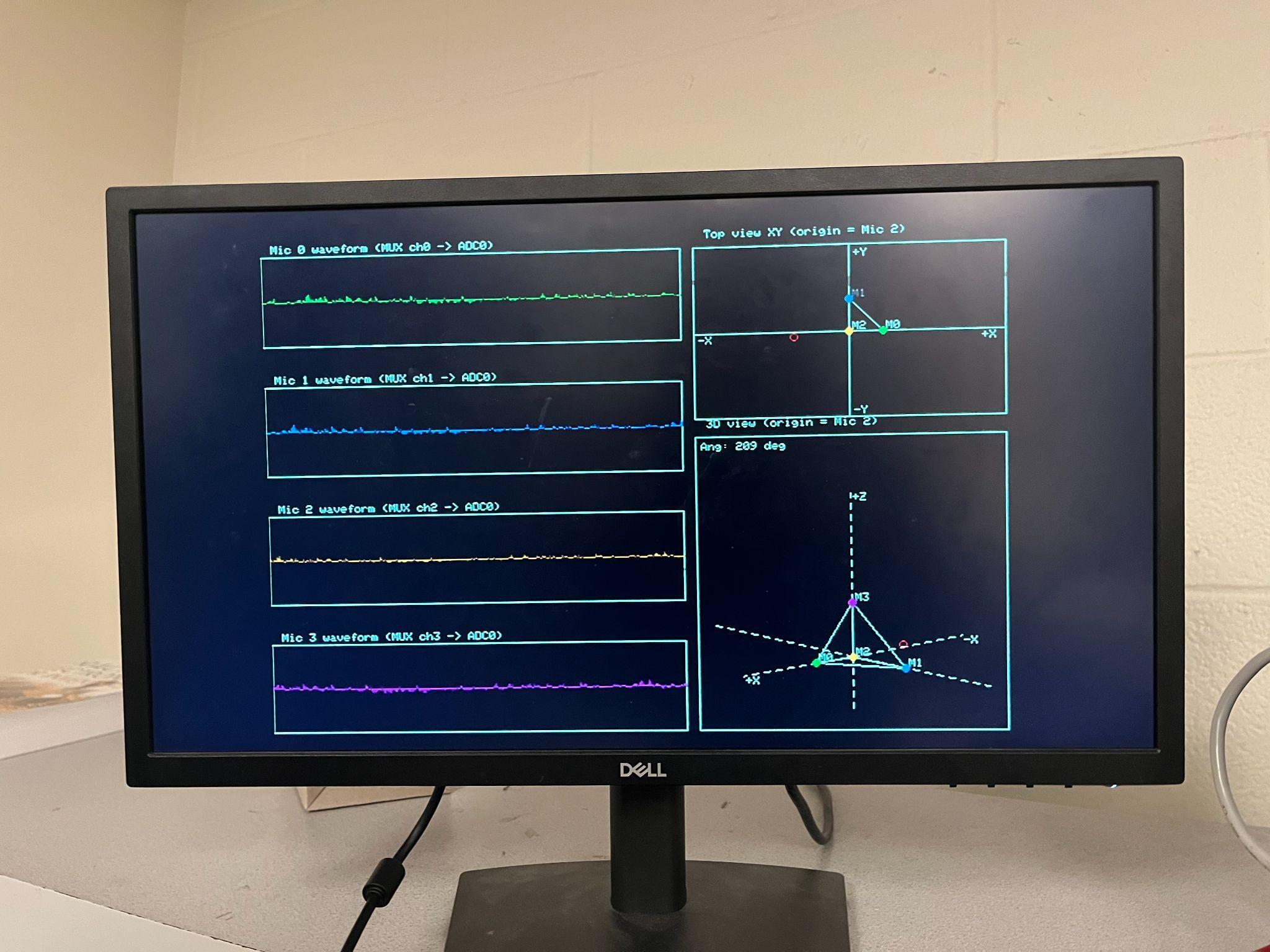
3D Audio Localization
[Fall 2025] We designed a real-time embedded system that localizes sound sources in three dimensions and visualizes them live using a four-m...
View project